nLab partial trace quantum channel

Contents

Context

Quantum systems

quantum logic


quantum physics


quantum probability theoryobservables and states


quantum information


quantum computation

qbit

quantum algorithms:


quantum sensing


quantum communication

Contents

Idea

For \mathscr{B} a finite-dimensional Hilbert space, the operation of partial trace over \mathscr{B} is a quantum channel

* * trace * |ψ,ββ,ψ| |ψβ|βψ|. \array{ \mathscr{H} \otimes \mathscr{B} \otimes \mathscr{B}^\ast \otimes \mathscr{H}^\ast & \xrightarrow{ trace^{\mathscr{B}} } & \mathscr{H} \otimes \mathscr{H}^\ast \\ \left\vert \psi, \beta \right\rangle \left\langle \beta', \psi' \right\vert &\mapsto& \left\vert \psi \right\rangle \left\langle \beta' \vert \beta \right\rangle \left\langle \psi' \right\vert \mathrlap{\,.} }

which represents the “operation” of averaging the mixed quantum states of the composite quantum system \mathscr{H} \otimes \mathscr{B} over the degrees of freedom of \mathscr{B}.

Properties

Environmental representation of quantum channels

The crux of dynamical quantum decoherence is that fundamentally the (time-)evolution of any quantum system \mathscr{H} may be assumed unitary (say via a Schrödinger equation) when taking the whole evolution of its environment \mathscr{B} (the “bath”, ultimately the whole observable universe) into account, too, in that the evolution of the total system \mathscr{H} \otimes \mathscr{B} is given by a unitary operator

evolve: |ψ,β U tot|ψ,β, \array{ \mathllap{ evolve \;\colon\; } \mathscr{H} \otimes \mathscr{B} &\longrightarrow& \mathscr{H} \otimes \mathscr{B} \\ \left\vert \psi, \beta \right\rangle &\mapsto& U_{tot} \left\vert \psi, \beta \right\rangle \mathrlap{\,,} }

after understanding the mixed states ρ: *\rho \,\colon\, \mathscr{H} \otimes \mathscr{H}^\ast (density matrices) of the given quantum system as coupled to any given mixed state env: *env \,\colon\, \mathscr{B} \otimes \mathscr{B}^\ast of the bath (via tensor product)

couple: * ()() * ρ ρenv; \array{ \mathllap{ couple \;\colon\; } \mathscr{H} \otimes \mathscr{H}^\ast & \longrightarrow & (\mathscr{H} \otimes \mathscr{B}) \otimes (\mathscr{H} \otimes \mathscr{B})^\ast \\ \rho &\mapsto& \rho \otimes env \mathrlap{\,;} }

…the only catch being that one cannot — and in any case does not (want or need to) — keep track of the precise quantum state of the environment/bath, instead only of its average effect on the given quantum system, which by the rule of quantum probability is the mixed state that remains after the partial trace over the environment:

(1)average:()() * * ρ^ Tr (ρ^). \array{ \mathllap{ average \;\colon\; } (\mathscr{H} \otimes \mathscr{B}) \otimes (\mathscr{H} \otimes \mathscr{B})^\ast &\longrightarrow& \mathscr{H} \otimes \mathscr{H}^\ast \\ \widehat{\rho} &\mapsto& Tr_{\mathscr{B}}\big(\widehat{\rho}\big) \mathrlap{\,.} }

In summary this means for practical purposes that the probabilistic evolution of quantum systems \mathscr{H} is always of the composite form

* couple to environment ( )( ) * total unitary evolution ( )( ) * average over environment * ρ ρenv U tot(ρenv)U tot Tr (U tot(ρenv)U tot ) \array{ \mathscr{H} \otimes \mathscr{H}^\ast & \xrightarrow{ \array{ \text{couple to} \\ \text{environment} } } & \left( \array{ \mathscr{H} \\ \otimes \\ \mathscr{B} } \right) \otimes \left( \array{ \mathscr{H} \\ \otimes \\ \mathscr{B} } \right)^\ast & \xrightarrow{ \array{ \text{total unitary} \\ \text{evolution} } } & \left( \array{ \mathscr{H} \\ \otimes \\ \mathscr{B} } \right) \otimes \left( \array{ \mathscr{H} \\ \otimes \\ \mathscr{B} } \right)^\ast & \xrightarrow{ \array{ \text{average over} \\ \text{environment} } } & \;\;\;\; \mathscr{H} \otimes \mathscr{H}^\ast \\ \rho &\mapsto& \rho \otimes env &\mapsto& \mathclap{ U_{tot} \cdot (\rho \otimes env) \cdot U_{tot}^\dagger } &\mapsto& \;\;\;\;\;\;\;\;\;\;\;\; \mathclap{ Tr_{\mathscr{B}} \big( U_{tot} \cdot (\rho \otimes env) \cdot U_{tot}^\dagger \big) } }

This composite turns out to be a “quantum channel

The realization of a quantum channel in the form (2) is also called an environmental representation (eg. Życzkowski & Bengtsson 2004 (3.5)).

In fact all quantum channels on a fixed Hilbert space have such an evironmental representation:

Proposition

(environmental representation of quantum channels)

Every quantum channel

chan: * * chan \;\;\colon\;\; \mathscr{H} \otimes \mathscr{H}^\ast \longrightarrow \mathscr{H} \otimes \mathscr{H}^\ast

may be written as

  1. a unitary quantum channel, induced by a unitary operator U tot:U_{tot} \,\colon\, \mathscr{H} \otimes \mathscr{B} \to \mathscr{H} \otimes \mathscr{B}

  2. on a compound system with some \mathscr{B} (the “bath”), yielding a total system Hilbert space \mathscr{H} \otimes \mathscr{B} (tensor product),

  3. and acting on the given mixed state ρ\rho coupled (tensored) with any pure state of the bath system,

  4. followed by partial trace (averaging) over \mathscr{B} (leading to decoherence in the remaining state)

in that

(2)chan(ρ)=Tr (U tot(ρenv)U tot ). chan(\rho) \;\;=\;\; Tr_{\mathscr{B}} \big( U_{tot} \cdot (\rho \otimes env) \cdot U_{tot}^\dagger \big) \,.

Conversely, every operation of the form (2) is a quantum channel.

This is originally due to Lindblad 1975 (see top of p. 149 and inside the proof of Lem. 5). For exposition and review see: Nielsen & Chuang 2000 §8.2.2-8.2.3. An account of the infinite-dimensional case is in Attal, Thm. 6.5 & 6.7. These authors focus on the case that the environment is in a pure state, the (parital) generalization to mixed environment states is discussed in Bengtsson & Życzkowski 2006 pp. 258.

Proof

We spell out the proof assuming finite-dimensional Hilbert spaces. (The general case follows the same idea, supplemented by arguments that the following sums converge.)

Now given a completely positive map:

chan: * *, chan \,\colon\, \mathscr{H} \otimes \mathscr{H}^\ast \longrightarrow \mathscr{H} \otimes \mathscr{H}^\ast \,,

then by operator-sum decomposition there exists a set (finite, under our assumptions) inhabited by at least one element

s ini:S, s_{ini} \,\colon\, S \,,

and an SS-indexed set of linear operators

(3)s:SE s:,withsE s E s=Id, s \,\colon\, S \;\;\; \vdash \;\;\; E_s \;\colon\; \mathscr{H} \longrightarrow \mathscr{H} \,,\;\;\;\; \text{with} \;\;\;\; \underset{s}{\sum} E_s^\dagger \cdot E_s \,=\, Id \mathrlap{\,,}

such that

chan(ρ)=sE sρE s . chan(\rho) \;=\; \underset{s}{\sum} \, E_s \cdot \rho \cdot E_s^\dagger \,.

Now take

S \mathscr{B} \,\equiv\, \underset{S}{\oplus} \mathbb{C}

with its canonical Hermitian inner product-structure with orthonormal linear basis (|s) s:S\big(\left\vert s \right\rangle\big)_{s \colon S} and consider the linear map

V: |ψ sE s|ψ|s. \array{ \mathllap{ V \;\colon\;\; } \mathscr{H} &\longrightarrow& \mathscr{H} \otimes \mathscr{B} \\ \left\vert \psi \right\rangle &\mapsto& \underset{s}{\sum} \, E_s \left\vert \psi \right\rangle \otimes \left\vert s \right\rangle \mathrlap{\,.} }

Observe that this is a linear isometry

ψ|V V|ψ =s,sψ|E s E s|ψs|sδ s s =ψ|sE s E sId|ψ =ψ|ψ. \begin{array}{ll} \left\langle \psi \right\vert V^\dagger V \left\vert \psi \right\rangle \\ \;=\; \underset{s,s'}{\sum} \left\langle \psi \right\vert E_{s'}^\dagger E_s \left\vert \psi \right\rangle \underset{ \delta_s^{s'} }{ \underbrace{ \left\langle s' \vert s \right\rangle } } \\ \;=\; \left\langle \psi \right\vert \underset{ Id }{ \underbrace{ \underset{s}{\sum} E_{s}^\dagger E_s } } \left\vert \psi \right\rangle \\ \;=\; \left\langle \psi \vert \psi \right\rangle \mathrlap{\,.} \end{array}

This implies that VV is injective so that we have a direct sum-decomposition of its codomain into its image and its cokernel orthogonal complement, which is unitarily isomorphic to dim()1dim(\mathscr{B})-1 summands of \mathscr{H} that we may identify as follows:

V()((|s 0)). \mathscr{H} \otimes \mathscr{B} \;\simeq\; V\big( \mathscr{H} \big) \oplus \Big( \mathscr{H} \otimes \big( \mathscr{B} \ominus \mathbb{C}\left\vert s_0 \right\rangle \big) \Big) \,.

In total this yields a unitary operator

U:((|s ini))V()((|s ini)) U \;\colon\; \mathscr{H} \otimes \mathscr{B} \,\simeq\, \mathscr{H} \oplus \Big( \mathscr{H} \otimes \big( \mathscr{B} \ominus \mathbb{C}\left\vert s_{ini} \right\rangle \big) \Big) \underoverset{}{}{\longrightarrow} V\big( \mathscr{H} \big) \oplus \Big( \mathscr{H} \otimes \big( \mathscr{B} \ominus \mathbb{C}\left\vert s_{ini} \right\rangle \big) \Big) \;\simeq\; \mathscr{H} \otimes \mathscr{B}

and we claim that this has the desired action on couplings of the \mathscr{H}-system to the pure bath state |s ini\left\vert s_{ini} \right\rangle:

trace (U(|s iniρs ini|)U ) =s,strace (|sE sρE s s|) =s,ss|sδ s sE sρE s =sE sρE s =chan(ρ). \begin{array}{l} trace^{\mathscr{B}} \Big( U \big( \left\vert s_{ini} \right\rangle \rho \left\langle s_{ini} \right\vert \big) U^\dagger \Big) \\ \;=\; \underset{s,s'}{\sum} trace^{\mathscr{B}} \big( \left\vert s \right\rangle E_s \cdot \rho \cdot E_{s'}^\dagger \left\langle s' \right\vert \big) \\ \;=\; \underset{s,s'}{\sum} \underset{ \delta_{s}^{s'} }{ \underbrace{ \left\langle s' \vert s \right\rangle } } E_s \cdot \rho \cdot E_{s'}^\dagger \\ \;=\; \underset{s}{\sum} E_s \cdot \rho \cdot E_{s}^\dagger \\ \;=\; chan(\rho) \,. \end{array}

This concludes the construction of an environmental representation where the environment is in a pure state.

Remark

The above theorem is often phrased as “… and the environment can be assumed to be in a pure state”. But in fact the proof crucially uses the assumption that the environment is in a pure state. It is not clear that there is a proof that works more generally.

In fact, if the environment is taken to be in the maximally mixed state, then the resulting quantum channels are called noisy operations or unistochastic quantum channels and are not expected to exhaust all quantum channels.

Environmental representation of measurement channels

By the general theorem about environmental representations of quantum channels, every quantum channel on a quantum system \mathscr{H} may be decomposed as

  1. coupling of \mathscr{H} to an environment/bath system \mathscr{B},

  2. unitary evolution of the composite system \mathscr{H} \otimes \mathscr{B},

  3. averaging the result over the environment states.

The way this works specifically for quantum measurement channels has precursor discussion von Neumann 1932 §VI.3 and received much attention in discussion of quantum decoherence following Zurek 1981 and Joos & Zeh 1985 (independently and apparently unkowingly of the general discussion of environmental representations in Lindblad 1975).
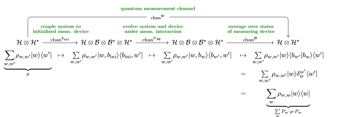
Concretely,

(we shall restrict attention to finite-dimensional Hilbert spaces not to get distracted by technicalities that are irrelevant to the point we are after)

if |b ini:\left\vert b_{\mathrm{ini}} \right\rangle \,\colon\, \mathscr{B} (we use bra-ket notation) denotes the initial state of a “device” quantum system then any notion of this device measuring the given quantum system \mathscr{H} (in its measurement basis WW, W\mathscr{H} \simeq \underset{W}{\oplus}\mathbb{C}) under their joint unitary quantum evolution should be reflected in a unitary operator under [[Zurek 1981 (1.1), Joos & Zeh 1985 (1.1.), following von Neumann 1932 §VI.3, review includes Schlosshauer 2007 (2.51)]]:

  1. the system \mathscr{H} remains invariant if it is purely in any eigenstate |w\left\vert w \right\rangle of the measurement basis,

  2. while in this case the measuring system evolves to a corresponding “pointer state” |b w\left\vert b_w \right\rangle:

(4) unitary measurement interaction U W: |w,b ini |w,b w \array{ &\mathclap{ \color{green} \array{ \text{unitary} \\ \text{measurement interaction} } }& \\ \mathllap{ U_W \;\colon\;\; } \mathscr{H} \otimes \mathscr{B} &\longrightarrow& \mathscr{H} \otimes \mathscr{B} \\ \left\vert w, b_{ini} \right\rangle &\mapsto& \left\vert w, b_w \right\rangle }

for b inib_{\mathrm{ini}} and b wb_w distinct elements of an (in practice: approximately-)orthonormal basis for \mathscr{B}. (There is always a unitary operator with this mapping property (4), for instance the one which moreover maps |w,b w|w,b ini\left\vert w, b_{w}\right\rangle \mapsto \left\vert w, b_{\mathrm{ini}}\right\rangle and is the identity on all remaining basis elements.)

But then the composition of the corresponding unitary quantum channel with the averaging channel over \mathscr{B} is indeed equal to the WW-measurement quantum channel on \mathscr{H} (cf. eg. Schlosshauer 2007 (2.117), going back to Zeh 1970 (7)), as follows:

Last revised on September 24, 2023 at 16:04:54. See the history of this page for a list of all contributions to it.